In this post, I want to explore RECAP(RL with Experience and Corrections via Advantage-conditioned Policies) which incorporates advantage estimation with imitation learning like actor-critic method in RL. In RECAP algorithm, advantage of actions are calculated through value network and feed this information into VLM backbone as improvement indicator. I believe that’s the overall concept of this method. However, this simple idea addresses the fundamental problem of combining RL with flow matching.
To begin with, I will first explain why you to know why we need RL in the pi 0.6 model and why combining RL with pi 0.6 was challenging. On top of that, I want to talk about the details of this method through equations.
Why RL?
In the field of Physical Intelligence, pretrained models have shown performance improvements in a number of tasks such as folding a laundry and assemble a box. Even so, pretraining + fine tune strategy was highly sensitive to the environment setting while having performance ceiling. In addition to that, if the robot encounters an unseen observations, it is susceptible to distribution shift due to the lack of data. However, applying RL can overcome these problems with human-intervention and self-experience. This is because that RL method can collect and learn from existing policy and human intervention.
Difficulties in RL + flow matching approach
To understand why the flow matching is hard to combine with RL, we need to understand the most popular RL method’s approach.
Probability distribution
PPO and SAC are the most common method in RL, and below is the key equations in these two algorithms. As you can verify, they needs $ \pi_{\theta}(a_t \mid s_t) $, which is the action distribution given by state $s_t$.
-
\(L^{CPI}(\theta) = \hat{\mathbb{E}}_{t} \left[ \frac{\pi_{\theta}(a_{t} \mid s_{t})}{\pi_{\theta_{\mathrm{old}}}(a_{t} \mid s_{t})} \hat{A}_{t} \right] = \hat{\mathbb{E}}_{t} \left[ r_{t}(\theta) \hat{A}_{t} \right]\)
PPO’s loss function -
\(J_{\pi}(\phi)=\mathbb{E}_{s_{t}\sim\mathcal{D}}[\mathbb{E}_{a_{t}\sim\pi_{\phi}}[\alpha \log(\pi_{\phi}(a_{t}|s_{t}))-Q_{\theta}(s_{t},a_{t})]]\)
SAC’s objective function
As you already know, flow matching method generates continuous actions through integration and it is not efficient to compute exact action log-probability. This is the primary reason why simple RL + flow matching does not work.
Theoretical details of RECAP
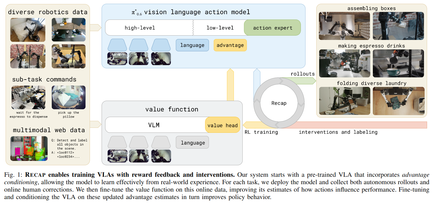
However, the authors proposed a straightforward approach to avoid this problem. They just implemented value network and they labeled actions as “positive” or “negative” with this value network. To be more precise, value network returns value which is the expected cumulative sum of rewards, and calculate advantage(how good the action is compared to expected value), and, finally, it categorizes the top 30% of advantages as positive and the bottom 30% as negative, passing this signal to the vlm backbone.
To train this value function they used reward function like below. I also note that success and failure are decided by human. $-C_{\text{fail}}$ is a large enough negative value so that the value can be distinguished from positive observation, and the agent receives a -1 reward at every step to encourage reaching the goal as quickly as possible.
\[r_t = \begin{cases} 0 & \text{if } t = T \text{ and success} \\ -C_{\text{fail}} & \text{if } t = T \text{ and failure} \\ -1 & \text{otherwise.} \end{cases}\]When they calculate the value function, they used distributional value function. It’s slightly different from a standard value function which returns a real number. They divided values into $B = 201$ bins and trained the value function like a bin classifier, and to calculate the real value it calculates expected value. The detailed equations are as follows.
\[\begin{flalign} & \min_{\phi} \mathbb{E}_{\tau \in \mathcal{D}} \left[ \sum_{\mathbf{o}_{t} \in \tau} H(R_{t}^{B}(\tau), p_{\phi}(V \mid \mathbf{o}_{t}, \ell)) \right] \\ & V(\mathbf{o}_{t}, \ell) = \sum_{b=1}^{B} p_{\phi}(V=b \mid \mathbf{o}_{t}, \ell) \cdot v(b) \\ & v(b) = V_{\min} + (b - 1) \frac{V_{\max} - V_{\min}}{B - 1} \quad \text{for } b \in \{1, 2, \dots, B\} \end{flalign}\]Once the value function is trained, advantages are computed and the top 30% are labeled as “positive”.
\[A^{\pi}(\mathbf{o}_t, \mathbf{a}_t) = \mathbb{E}_{\rho_{\pi}(\tau)} \left[ \sum_{t'=t}^{t+N-1} r_{t'} + V^{\pi}(\mathbf{o}_{t+N}) \right] - V^{\pi}(\mathbf{o}_t)\]By labeling observations as positive or negative, the model learns to distinguish good actions from bad ones without computing explicit action log-probabilities. In conclusion, RECAP elegantly circumvents the core incompatibility between flow matching and standard RL objectives.
Real application of RECAP
\begin{algorithm}
\caption{RL with Experience and Corrections via Advantage-conditioned Policies (RECAP)}
\begin{algorithmic}
\REQUIRE multi-task demonstration dataset $\mathcal{D}_{\text{demo}}$
\STATE Train $V_{\text{pre}}$ on $\mathcal{D}_{\text{demo}}$ using Eq. 1
\STATE Train $\pi_{\text{pre}}$ on $\mathcal{D}_{\text{demo}}$ using Eq. 3 and $V_{\text{pre}}$
\STATE Initialize $\mathcal{D}_\ell$ with demonstrations for $\ell$
\STATE Train $V_\ell^0$ from $V_{\text{pre}}$ on $\mathcal{D}_\ell$ using Eq. 1
\STATE Train $\pi_\ell^0$ from $\pi_{\text{pre}}$ on $\mathcal{D}_\ell$ using Eq. 3 and $V_\ell^0$
\FOR{$k = 1$ to $K$}
  \STATE Collect data with $\pi_\ell^{k-1}$, add it to $\mathcal{D}_\ell$
  \STATE Train $V_\ell^k$ from $V_{\text{pre}}$ on $\mathcal{D}_\ell$ using Eq. 1
  \STATE Train $\pi_\ell^k$ from $\pi_{\text{pre}}$ on $\mathcal{D}_\ell$ using Eq. 3 and $V_\ell^k$
\ENDFOR
\end{algorithmic}
\end{algorithm}
The algorithm starts with training value network in the pretraining data, and train the policy. After that, it fine-tunes both the value function and policy for each task. Then in the for loop with k they collect more data with the policy while intervening bad actions by human. In the collecting process in the loop, robots collect data with their policy but a human corrects the robot’s actions when they appear unsafe or clearly wrong.
In line 7, human interventions are always labeled as positive, under the assumption that actions provided by a human are correct and other actions that the policy has generated are classified with advantage function and if it’s in 30%, actions are positive. Otherwise, actions are negative.
Conclusion
At first glance, I thought that it’s not like RL since it pretrains policy with imitation learning and, even at the last, collecting data contains human intervention. On top of that, it’s not a reward maximizing algorithm. Reward function is just for value function training. I believe that it explains how hard to reach a goal without guidance of human. With full RL method like PPO and SAC, humanoid walking environment can be solved with motion which is far from natural human gait. In the case of robotics, their tasks like pick&place and folding laundry are very difficult compared to walking, and they give very sparse rewards since the reward is only provided when the task is done. As a result, researchers have made sophisticated imitation learning method inspired by RL method, and fully automated data collecting and training loop is the future challenge humanity must solve for general-purpose robotic systems.
References
-
Physical Intelligence et al., “$\pi^{*}_{0.6}$: a VLA That Learns From Experience,” arXiv:2511.14759, 2025. https://arxiv.org/abs/2511.14759
-
Schulman, J., Wolski, F., Dhariwal, P., Radford, A., and Klimov, O., “Proximal Policy Optimization Algorithms,” arXiv:1707.06347, 2017. https://arxiv.org/abs/1707.06347
-
Haarnoja, T., Zhou, A., Hartikainen, K., Tucker, G., Ha, S., Tan, J., Kumar, V., Zhu, H., Gupta, A., Abbeel, P., and Levine, S., “Soft Actor-Critic Algorithms and Applications,” arXiv:1812.05905, 2018. https://arxiv.org/abs/1812.05905